INTRODUCTION
A CFRP panel made to the specification of a Federal Aviation Administration (FAA) NDI Proficiency specimen 2A was manufactured to benchmark the capabilities of the dolphicam2.
The material and the thickness of the panel are representative of the solid laminate composites on commercial aircraft such as Boeing 787 and Airbus A350. On these aircraft, such a laminate is used as the primary structural material of most of the fuselage and wing surfaces. This panel features various manufacturing flaws typical of aerospace composites, and as such is used to assess the performance of NDT equipment and to train NDI personnel. The panel is a 24 ply co-cured substructure (16 ply skin with 8 ply stiffeners and built-up pads). This corresponds to a nominal thickness over the majority of the panel of 0.12″ and a maximum thickness of ~0.3″. The panel is 24″×18″ and its geometry is designed to include a wide range of common flaws in this relatively compact area.
The flaws present include missing sealant, pillow inserts, Dremel cut, flat bottom holes, left-in prepreg backing, and grease. Photographs of both sides of the panel are shown in Figure 1.
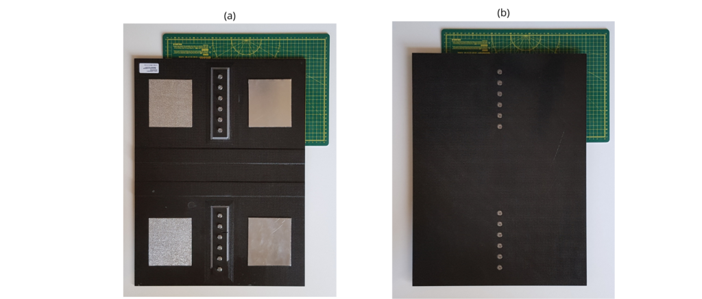
Figure 1. a) Photograph of the bottom face of the panel showing the ply build ups/sound dampers. b) Photograph of the top face of the panel (the “inspection side”).
The nominal locations of the manufactured flaws are shown in Figure 2. The labelled numbers in the figure correspond to the item numbers in Table 1. Figure 2 shows the panel from two orientations; it shows the face pictured in Figure 1a from the same orientation, and underneath this, a side profile of the panel. Further dimensions and details of the panel are given in Figure 3.
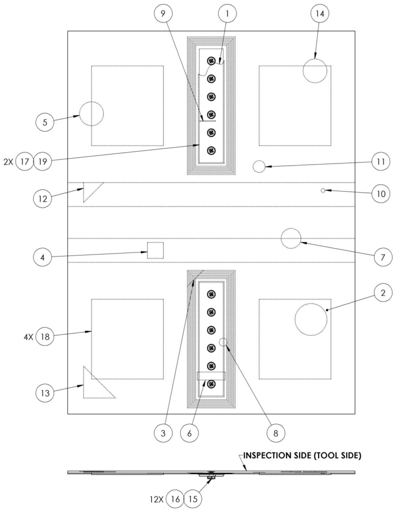
Figure 2. Technical drawing showing main features on the panel in their nominal locations.
Table 1. Nominal dimensions of panel features.
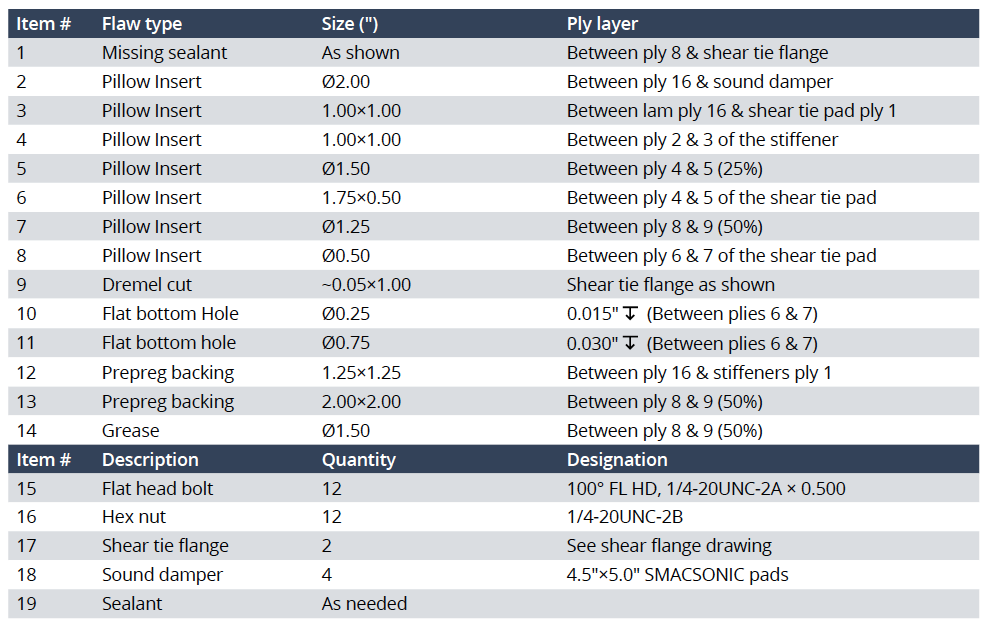
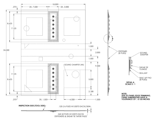
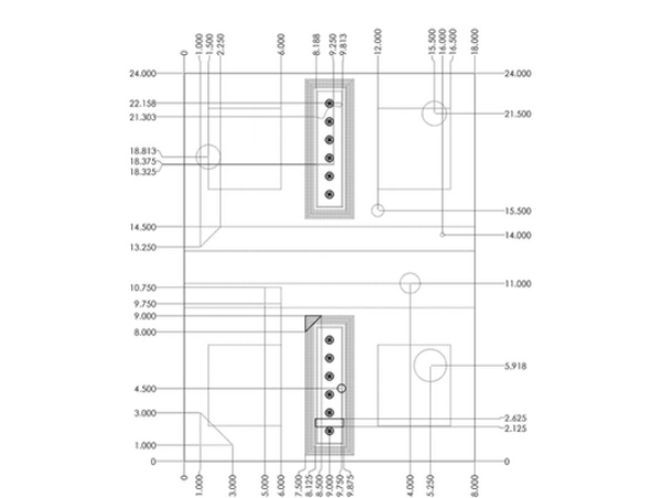
Figure 3. Technical drawings for the specification of the panel.
SOLUTION
The panel was inspected using a dolphicam2 and a TRM-CI-5MHz Transducer Module (TRM). This TRM is our mid-range frequency model, capable of penetrating the ~0.3″ maximum thickness of the panel reliably while still providing excellent resolution of flaws. A mixture of gel and water was used as a couplant to provide optimal sound transmission, however, with the Aqualene delay line of the TRM-CI-5MHz, water would be sufficient to ensure good coupling.
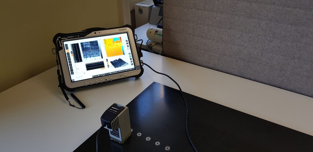
Figure 4. Photograph of dolphicam2 with TRM-CI-5MHz transducer on panel.
The flaws were located by freehand scanning the TRM over the entire panel and monitoring the software display. Where the flaws were located, a combination of single C-scans and manually stitched C-scans were acquired. For the final flaw (item 14), in addition to acquiring a manually stitched scan, an additional scan was acquired using an ODI – single probe wheel encoder. Both manual stitching and encoding are suitable methods for mapping a region greater than the aperture of the transducer, and produce very similar results. Encoding typically becomes the preferred option as mapping size increases, since the acquisition time is generally reduced.
With the dolphicam2, the amplitude and time of flight data are acquired simultaneously. In this study, the amplitude and time of flight data are plotted in the bone and jet colour schemes respectively, and the dimensions are set to inches to be consistent with the panel specifications.
FINDINGS
All flaws were successfully detected using the dolphicam2 with dimensions that are consistent with their nominal value. Scans from each flaw will be presented and discussed in turn.
Figure 5 shows the approximate locations of the identified flaws overlaid on a photograph of the panel, adjacent to a technical drawing showing the nominal locations of the flaws. Each yellow box on the photograph represents the approximate region where a C-scan was acquired. The acquired C-scans themselves are shown in Figures 6 to 16. The item numbers on the photograph are orientated based on the orientation of the C-scans.
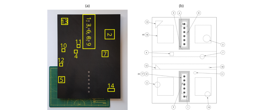
Figure 5. a) Photograph of the inspection side with an overlay of scan areas and corresponding item number(s) for the flaw(s) found within each scan area. The numbers are orientated based on the orientation of the scan. b) Technical drawing showing the location of flaws from the inspection side.
There are annotations on each scan showing the measurements taken, with the measurements summarised in Table 2. For item 14, which has both a manually stitched scan and an encoded scan, the measurements from the manually stitched scan will be used for consistency.
Figure 6 shows a mapped scan of one of the two shear tie structures present. This structure contains flaws labelled items 1, 3, 6, 8, 9. Item 1 is the missing sealant, which presents as a sharp discontinuity in the amplitude C-scan. This can be contrasted with the intact sealant which presents as a smooth transition at the edge of the shear tie flange.
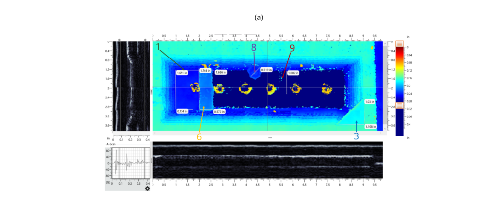
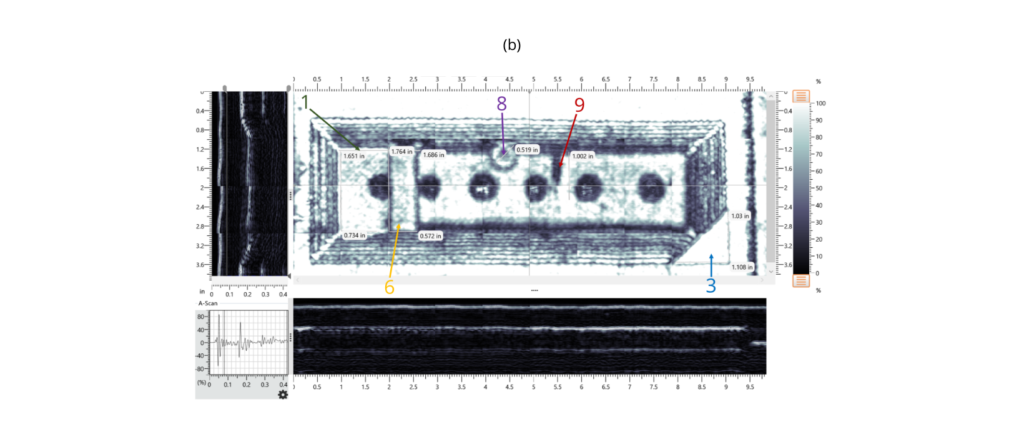
Figure 6. a) Manually stitched Amplitude C-scan with b) corresponding time of flight C-scan.
Items 3, 6 and 8 are pillow inserts, which can be seen as outlined shapes in the amplitude data and shapes at different depths in the time of flight data. Since item 3 is shallower within the panel from the inspection side (between lam ply 16 & shear tie pad ply 1 from Table 1), it appears as a turquoise colour in the time of flight corresponding to a depth of 0.13″ using a depth measure point on the C-scan. Items 6 and 8 are deeper into the laminate and thus are a blue colour. These were measured at depths of 0.17″ and 0.19″ for items 6 and 8 respectively using point markers. This is expected as item 6 is between ply 4 & 5 of the shear tie pad and item 8 is between ply 6 & 7 of the shear tie pad from Table 1.
The pillow inserts reflect the majority of the incident ultrasound before it can reach deeper locations, which can lead to the absence of details in the region directly below the inserts in both the amplitude and time of flight scans. This is particularly apparent for item 3 as its positioning between the 16-ply ply skin and the shear tie pad means the ultrasound is reflected before it can reach the step-like detail of the shear tie pad.
Also shown in Figure 6 is Item 9, a Dremel cut, which can be seen as a black feature in the amplitude data. This is because the cut angles do not present a reflective surface for the ultrasound. It has a more flecked appearance in time of flight data, but the presence of this change in texture helps to confirm the flaw.
Flaws 3, 6 and 8 appear to be in the correct positions, but 1 and 9 appear to be misplaced relative to their nominal locations. It appears they have been manufactured on the wrong shear tie structure and that item 6 is not meant to obscure item 1. The relative positions on the shear tie structure are correct and a visual check of the bottom face confirms that 1 and 9 have been manufactured on the incorrect shear tie structure and that the identification of their positions on the C-scan is correct. Nevertheless, the C-scan demonstrates that the flaws manufactured on the shear tie structure are easily identifiable using dolphicam2.
Subsequently, each scan will contain one flaw with the remaining flaw being presented in ascending order corresponding to its item number in Table 1. With this, Figures 7, 8 and 9 show items 2, 4 and 5. Items 2 and 5 can be seen as circular features, and item 4 appears as a rectangular feature. They are readily resolved in both the amplitude and time of flight data. Item 2 has a bar like indication running through the main circular indication and can be observed to be slightly deeper relative to the local back wall. Item 4 has a lower amplitude local back wall echo as it is located on the stiffener region which has a greater overall thickness. Item 5 can be seen to be closer to the surface on the inspection side and item 2 is the furthest due to their position in the B-scan and the time of flight scan. Also, using depth measure points on the C-scan results in values of 0.13″, 0.15″ and 0.05″ for items 2, 4 and 5 respectively (from Table 1, item 2 is between ply 16 & sound dampener, item 4 is between ply 2 & 3 of the stiffener, and item 5 is between ply 4 & 5).
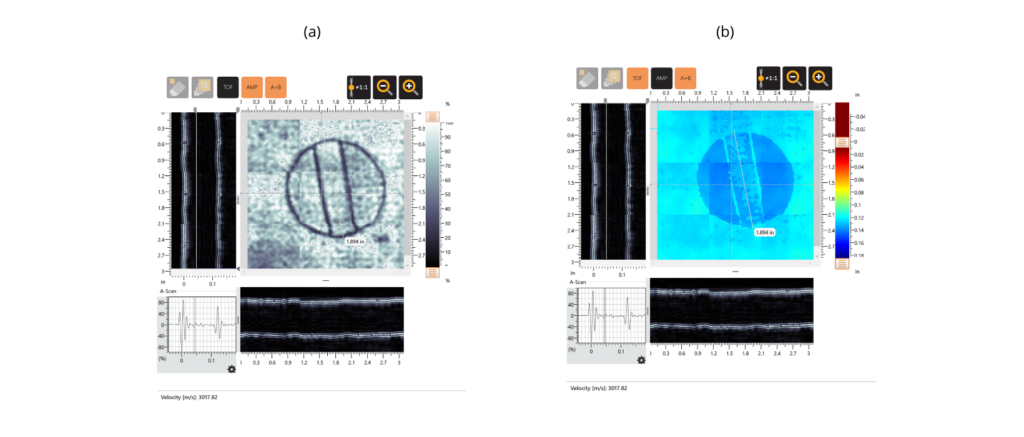
Figure 7. a) Manually stitched Amplitude C-scan with b) corresponding time of flight C-scan of flaw labelled item 2.
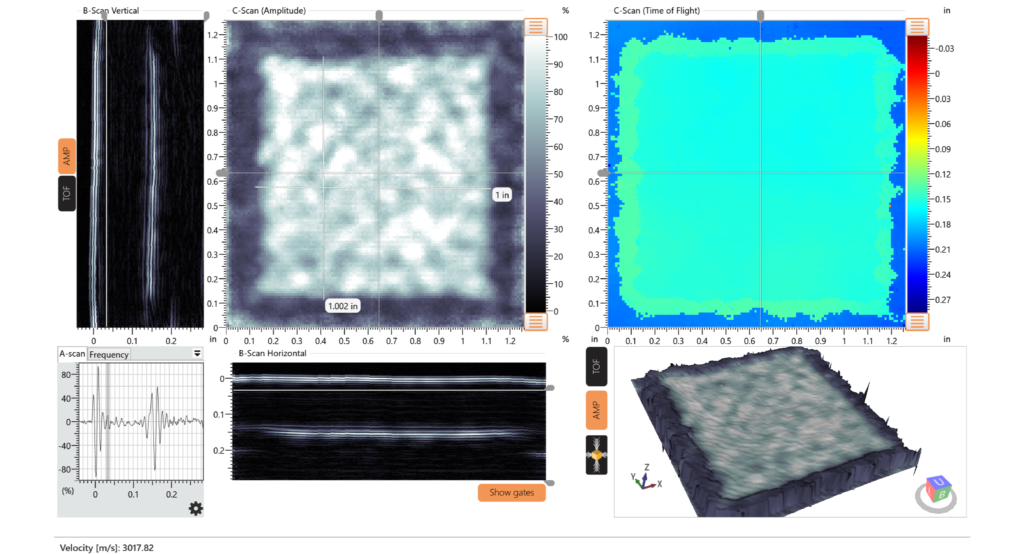
Figure 8. All view screenshot of flaw labelled item 4.
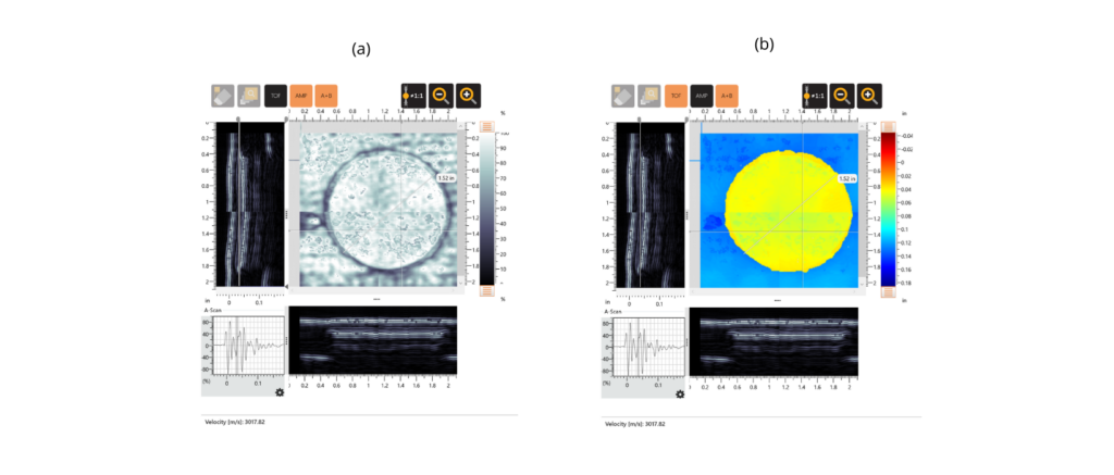
Figure 9. a) Manually stitched Amplitude C-scan with b) corresponding time of flight C-scan of flaw labelled item 5.
Another pillow insert (item 7) is shown in Figure 10. There is a stiffener behind half of the pillow insert, which creates a step-like feature behind the circular feature. This is more evident in the time of flight where it is visibly deeper. Again, the stiffener results in a lower amplitude back wall echo in the amplitude scan as the ultrasound is attenuated by the increase in material thickness.
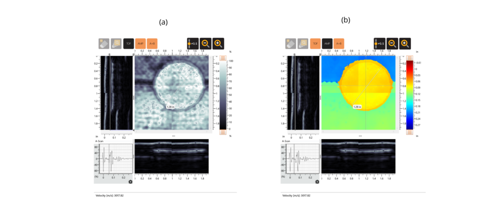
Figure 10. a) Manually stitched Amplitude C-scan with b) corresponding time of flight C-scan of flaw labelled item 7.
Flat bottom holes corresponding to items 10 and 11 are shown in Figures 11 and 12 respectively. Part of the scan in Figure 11 is on the stiffener, which can be seen as a lower amplitude back wall echo in the amplitude C-scan and a blue region in the time of flight C-scan. An additional inclusion was also observed in Figure 11, which was visible in both the amplitude and time of flight C-scans. The origin of this inclusion is unknown, but it could be a foreign particle or prepreg backing. Items 10 and 11 were in positions that differ from the nominal ones. As with the misplacement of the two other features (item numbers 1 and 9), this was visually confirmed by looking at the bottom face of the panel.
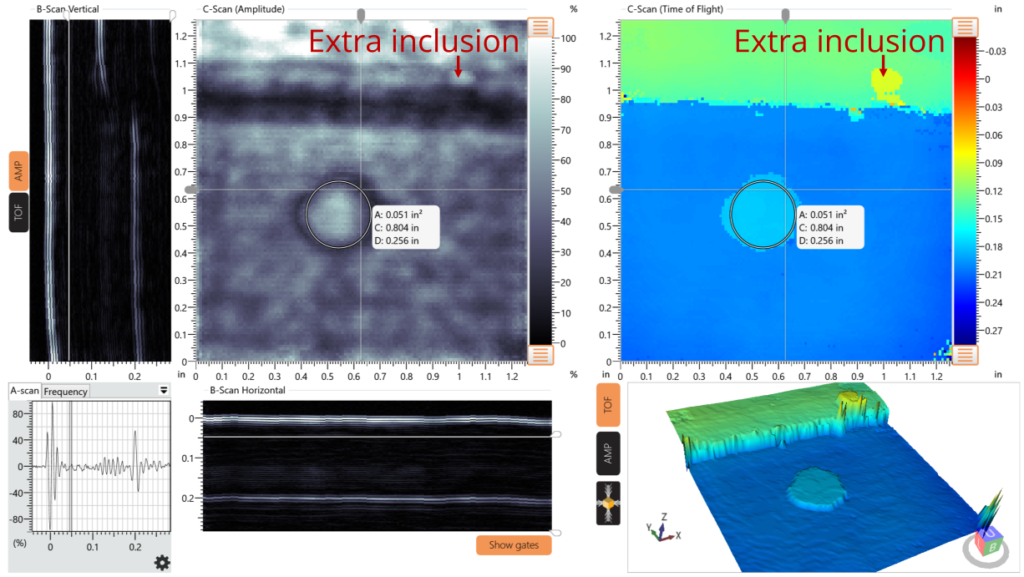
Figure 11. All view screenshot of flaw labelled item 10. It is possible to see an extra feature to the top right quadrant of the C-scans. This is clearest in the time of flight C-scan where it can be seen as a yellow feature.
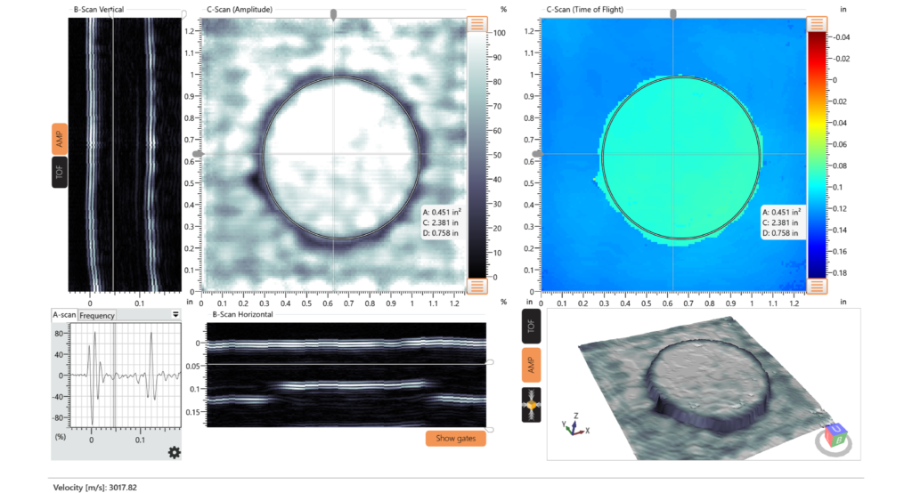
Figure 12. All view screenshot of flaw labelled item 11.
Figures 13 and 14 show the left-in prepreg backing flaws (items 12 and 13). Their appearance in the amplitude and time of flight scans is as expected and is consistent with their nominal location and expected signal amplitude. Along the bottom edge of item 12, there is a transition in thickness from being in the stiffener region to being off it.
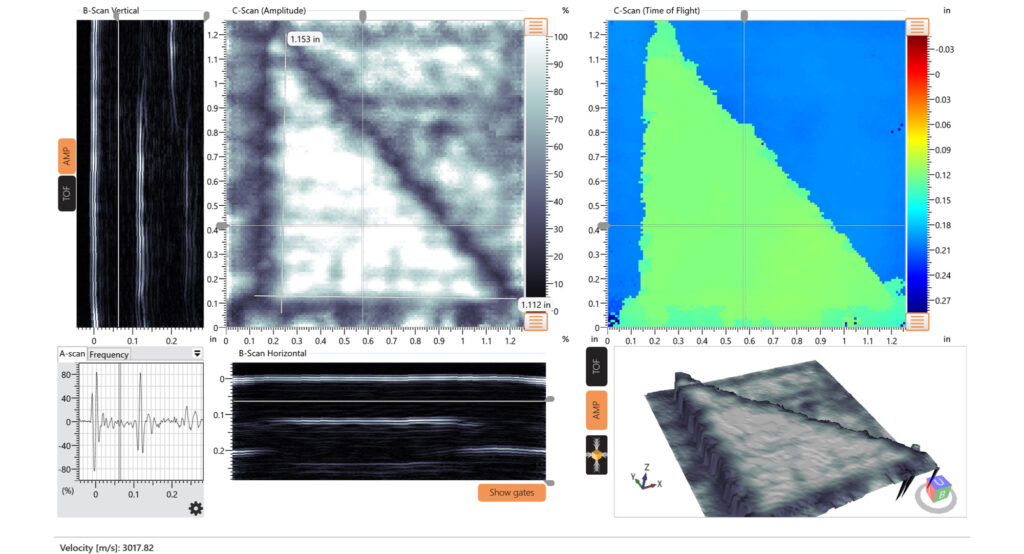
Figure 13. All view screenshot of flaw labelled item 12.
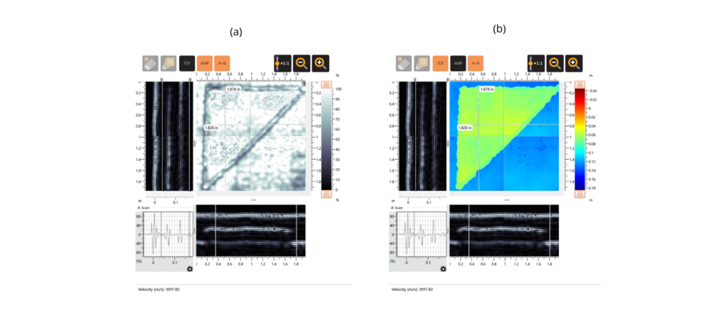
Figure 14. a) Manually stitched Amplitude C-scan with b) corresponding time of flight C-scan of flaw labelled item 13.
Both Figure 15 and 16 shows item 14, which is grease contamination. Figure 15, like the preceding figures, uses manual stitching for mapping, while Figure 16 uses an encoder (ODI – single probe). The results are almost identical, showing the ability to use either manual stitching or encoder scanning and produce consistent results.
It is clear from these scans that the grease has smeared during the consolidation of the laminate. There is a single main patch, which seems smeared in the vertical direction, surrounded by various smaller patches.
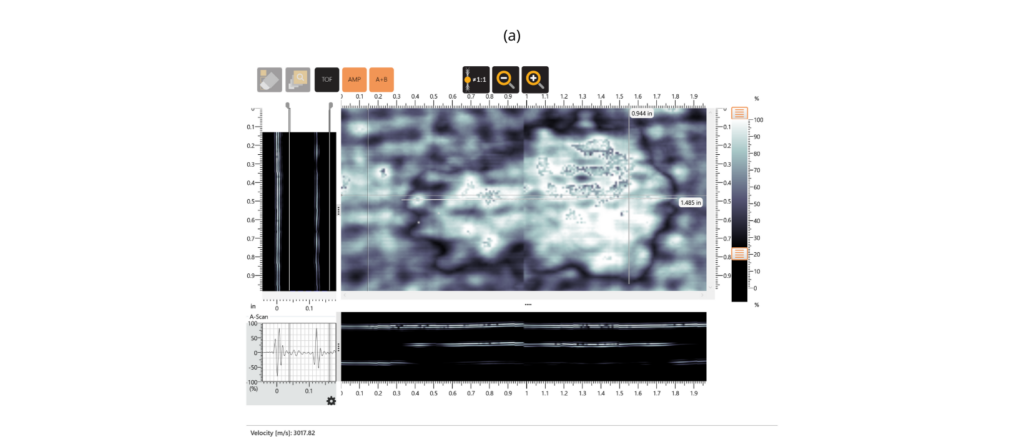
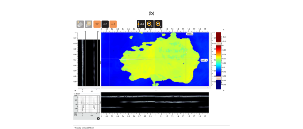
Figure 15. a) Manually stitched Amplitude C-scan with b) corresponding time of flight C-scan of flaw labelled item 14.
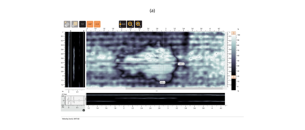
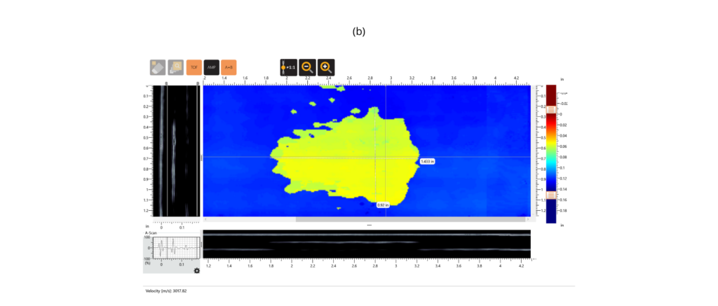
Figure 16. a) Encoded Amplitude C-scan with b) corresponding time of flight C-scan of flaw labelled item 14.
The C-scans of Figures 6 to 16 have demonstrated that all the flaws of interest can be clearly resolved and characterised using the dolphicam2. All flaws were found in the nominal locations except for four flaws (items 1, 9, 10 and 11). These four flaws are all the ones that are visible from the bottom face, and they could be confirmed to be misplaced.
With all flaws accounted for, the dimensional measurements for the flaws on each of the C-scans were compiled to form Table 2. The displayed precision of these values is reflective of full value from the measurement tool rather than actual precision, where the measurements are only taken roughly. Also in Table 2, the nominal sizes from Table 1 were repeated to allow them to be compared side-by-side, and the difference between the measured and nominal dimensions was given. For items where multiple dimensions are measured, the differences between each of the measured dimensions and their nominal counterpart are calculated then the average of these calculated values is given as the difference.
Table 2. Nominal and measured dimensions of flaws with the difference between them as a percentage.
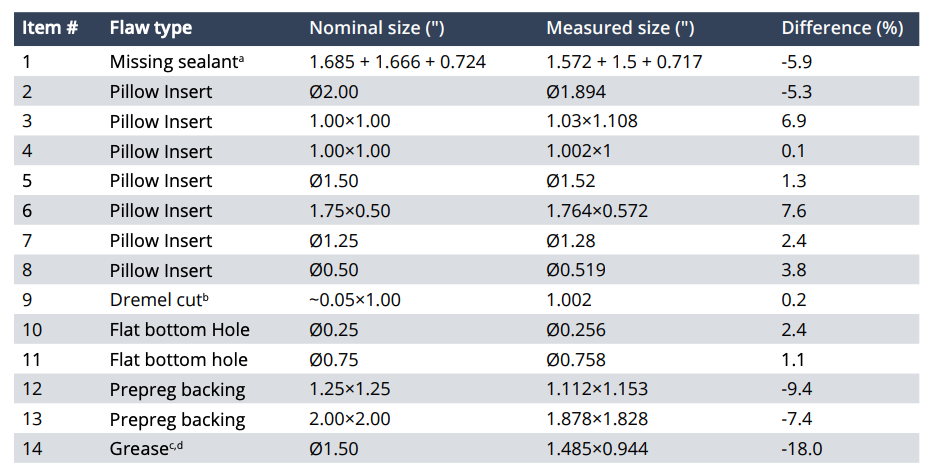
a) Nominal size of the missing sealant is calculated from the technical drawing since no nominal sizes are given explicitly.
b) The width of the Dremel indication is omitted as it was difficult to determine the width of such a thin cut accurately.
c) Two measurements instead of a single diameter reading are given since the indication is not circular. In this case, these two values are each compared to the nominal diameter for the “difference”.
d) Measurements from the manually stitched scan are used.
From Table 2, all the flaws were measured to be within 18.0% of their nominal dimensions with a mean difference of 1.4% and a mean absolute difference of 5.1%.
CONCLUSION
The dolphicam2 with a TRM-CI-5MHz transducer (TRM) was able to successfully inspect the FAA NDI Proficiency Specimen 2A. All the manufactured flaws were clearly resolved and characterised.
These flaws are categorised as missing sealant, pillow inserts, dremel cut, flat bottom holes, prepreg backing and grease. Moreover, the flaws could be sized, and they were found to be in good agreement with nominal dimensions. The time and cost savings enabled by the dolphicam2 is demonstrated by this ability to characterise such a wide range of flaw types with a single setup. The TRM-CI-5MHz transducer is versatile and well-suited for many aerospace applications featuring thin to moderate thicknesses of both composites and metals.

MxTTU
MxTTU™ makes the assessment of complex materials from multiple-bond layers to honeycomb or foam cores far simpler.
Transducers (TRMs)
TRM 5 MHz
The 5MHz transducer module (TRM) sits at the middle of our range and is a fantastic all-rounder.
Transducers (TRMs)
Dolphicam2
Pelicase includes a 10” rugged tablet, Black Box and cables for the dolphicam2
Core Units
MxTTU
MxTTU™ makes the assessment of complex materials from multiple-bond layers to honeycomb or foam cores far simpler.
Transducers (TRMs)
TRM 5 MHz
The 5MHz transducer module (TRM) sits at the middle of our range and is a fantastic all-rounder.
Transducers (TRMs)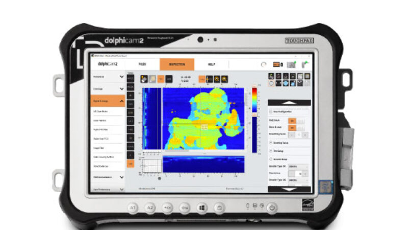
Dolphicam2
Pelicase includes a 10” rugged tablet, Black Box and cables for the dolphicam2
Core UnitsAEROSPACE MARKET
Dolphicam2 is certified by two of the world’s leading aircraft manufacturers – Boeing has authorised specific NDT procedures for their 787 aeroplanes, and Airbus has accepted the dolphicam2 for all composite inspections on its assets.
Read moreREQUEST A QUOTE OR SUBMIT AN ENQUIRY
Need help with product information?
Get in touch with our experts for information or a quotation.